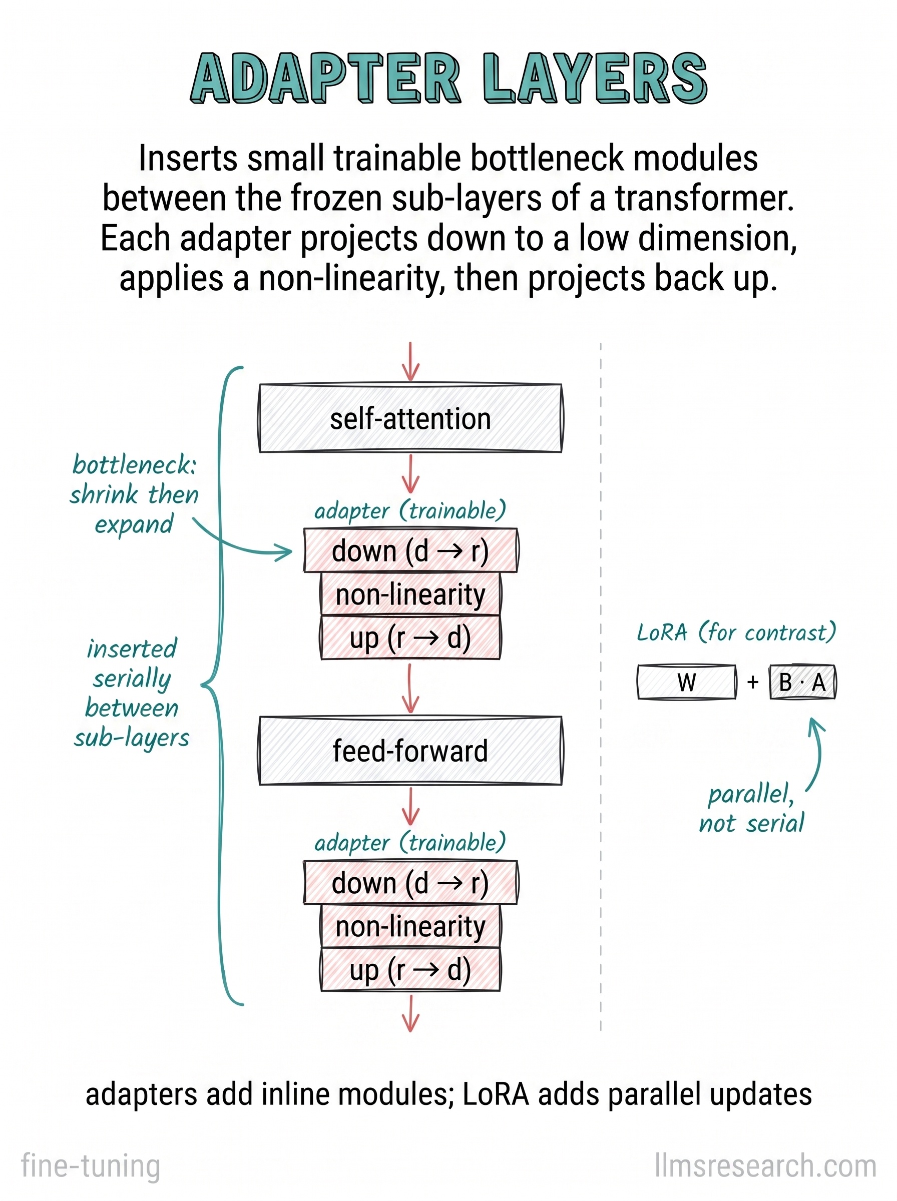
Adapter layers were an early PEFT design, and comparing them with LoRA sharpens what “where you insert the trainable parameters” actually means. The card shows a transformer layer with its self-attention and feed-forward sub-layers frozen, and a small adapter module inserted after each one, in the main data path. Each adapter is a bottleneck: it projects the d-dimensional activations down to a small dimension r, applies a non-linearity, then projects back up to d. Only these down and up projections are trained.
The bottleneck shape is what keeps the module cheap. Projecting to a small r and back means the added parameters scale with r rather than with d-squared, the same efficiency argument that motivates LoRA. The non-linearity in the middle is the one structural difference worth noting: because the adapter passes its reduced representation through a nonlinear function, it is not merely a low-rank linear update but a small nonlinear transformation of the activations.
The contrast the card draws on the right is the important one. LoRA is written as W plus B times A, placed in parallel with a frozen weight matrix, and labeled parallel, not serial. Adapters sit serially, inserted between sub-layers so every activation flows through them in sequence. That placement has a consequence at inference time. A LoRA update can be folded into the original weights by addition, so a merged model runs at the original speed, while a serial adapter is an extra computation in the forward path that cannot be absorbed away, adding a small but real latency to every token.
That inference cost is the main reason LoRA displaced adapters as the default even though both reach comparable quality. Adapters remain a clear illustration of the design space, and the caption sums up the distinction cleanly: adapters add inline modules, LoRA adds parallel updates. The next cards leave the question of where to put trainable parameters and turn to what can go wrong during fine-tuning regardless of the method.